import cv2, numpy as np
from matplotlib import pyplot as plt
from sklearn.datasets import fetch_olivetti_faces
from keras.models import Sequential
from keras.layers import Dense, MaxPooling2D, Flatten, Activation
from keras.layers.convolutional import Convolution2D
from sklearn.model_selection import train_test_split
import keras.utils as utils
import cv2
import keras
import io
import tensorflow.keras as tk
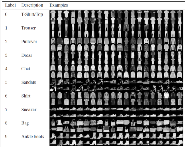
1. Fashion Item 구분
class_names = ['T-shirt/top', 'Trouser', 'Pullover', 'Dress', 'Coat',
               'Sandal', 'Shirt', 'Sneaker', 'Bag', 'Ankle boot']

(x_train, y_train), (x_test, y_test) = keras.datasets.fashion_mnist.load_data()
x_train, x_test = x_train / 255.0, x_test / 255.0
# 0에서 1로 정규화 시키는 것이 학습 속도를 빠르게 함

print(x_train.shape)
print(y_train.shape)
print(x_test.shape)
print(y_test.shape)
(60000, 28, 28) (60000,) (10000, 28, 28) (10000,)
plt.imshow(x_train[50], cmap='gray')
plt.title(class_names[y_train[50]])
x_train2 = x_train.reshape(-1, 28*28) #-1의 의미는 전체 샘플수를 1차원으로 크기 변경
x_test2 = x_test.reshape(-1, 28*28)
y_h = np.eye(10)[y_train] #ont-hot 인코딩
A = np.hstack([ x_train2, np.ones(( x_train2.shape[0]  ,1))  ]) #행뒤에 1로 이뤄진 컬럼을 붙임
print(A.shape) # +1 된값
print(A[0])
역행렬 기반 학습
역행렬을 이용해서 만들 때는 행렬을 사용해야한다.
2차원 데이터를 직접 이용할 수 없기 때문에 1차원으로 변경
(60000, 785)
A[0]을 출력해보면 맨 뒤에 1일 붙은 것을 확인 할 수 있음
%time #실행시킨 결과가 걸리는 시간
inv = np.linalg.pinv(A)
W = np.matmul(inv, y_h)
print(W.shape)
#W는 10개의 클래스를 구분하는 문제, 컬럼은 각각의 클래스에 해당하는 가중치가 된다.
#전체 w중 컬럼중에 첫번째 컬럼은 첫번째의 패션 아이템을 잘 구분할수 있는 가중 치,
#두번째 컬럼은 두번째 아이템을 잘 구분할수 있는 가중 치
(785, 10)
weight의 갯수 , 클래스의 수
print(W[0]) #10개의 클래스에서 첫번째 가중치
print(W[:, 0]) #785개의 w값, 0번째 클래스를 잘 분류할 수 있는 가중치
#테스트 데이터를 활용해서 인식성능 계산
A = np.hstack([ x_test2, np.ones(( x_test2.shape[0]  ,1))  ])
#테스트 데이터를 A행렬로 바꾼 다음에
predict = np.matmul(A, W)
#A와 W를 곱하면 predict 구할 수 있다.
print(predict.shape)
label = np.argmax(predict, axis=1) #확률값으로 부터 레이블로 바꿈, 최대값을 갖는 인덱스를 가져옴
print(label)
np.mean(label == y_test)
#예측된 값과 실제 레이블을 비교해서 평균을 구하면 평균 인식률임
(10000, 10) [9 2 1 ... 8 1 5]
0.8113
테스트 데이터가 10000개, 테스트 데이터 하나당 클래스 수가 10개
예측 값으로 부터 레이블 값 바꾸는 방법은 argmax 함수 사용
n = 10

predict = np.matmul(A[n], W)
#10번째 데이터를 예측

print(predict)
#10개의 클래스의 확률값이 나옴

id = np.argmax(predict) #가장 큰값을 찾음
#axis=1을 주지 않는 이유? 어짜피 하나의 데이터만 테스트를 해야하기 때문에,
#결과값이 벡터 이기 때문에 (벡터는 쓰나 안쓰나 동일)

print(id)

plt.subplot(1,2,1)
plt.bar(range(0,10), predict)
#x축은 0~10까지 , 확률값

plt.subplot(1,2,2)
plt.imshow(x_test[n], cmap='gray')
#실제 테스트 이미지를 출력

col =  "blue" if  y_test[n] == id else "red"
plt.title(f"T:{class_names[y_test[n]]}  P:{class_names[id]}", color = col)
#예측한 값과 정답이 같으면 파란색, 틀렸으면 빨간색
신경망 기반 학습
model = Sequential() #이전 출력을 다음 뉴런의 인풋으로 사용
model.add(Dense(256, activation='relu')) #256개의 노드로 구성된 은닉층
model.add(Dense(128, activation='relu')) #128개의 노드로 구성된 은닉층
model.add(Dense(10, activation='softmax')) #출력단, 실제 분류할 클래스로 맞춰줘야함
model.compile(loss='sparse_categorical_crossentropy', optimizer='adam', metrics=['accuracy'])
#sparse_categorical_crossentropy을 사용하는 이유 : 원핫 인코딩된 레이블을 사용하지 않고 학습 가능
%%time
hist = model.fit(x_train2, y_train, epochs = 10, batch_size=100)
plt.plot(hist.history['loss'])
plt.plot(hist.history['accuracy'])
학습 데이터에 대한 accuracy
model.evaluate(x_test2, y_test)
테스트 데이터로 인식률 구하기
→ 이전 인버스 문제로 풀었을 때 보다 성능이 개선되었다.
CNN 기반 학습
x_train3 = x_train.reshape(-1,28,28,1) #input을 4차원 데이터로 넣어준다.
x_test3 = x_test.reshape(-1,28,28,1)
샘플수, 2d이미지의 폭과 높이, 1(흑백) or 3(컬러)
<CNN구축과정>
model = Sequential()
model.add(Convolution2D(32, (3, 3), padding='same',
input_shape=x_train3.shape[1:]))
#컨볼루션 레이어, 32개의 필터, 커널의 크기는 3*3, 제로 패딩, 1이후의 형태로 인풋 데이터가 주어짐
model.add(Activation('relu'))
#활성화 함수를 거침
model.add(MaxPooling2D(pool_size=(2, 2)))
#맥스 풀링 레이어, 영상의 크기를 2배로 줄임
model.add(Convolution2D(64, (3, 3), padding='same'))
#필터수를 32->64개로 늘림, 일반적으로 cnn은 필터를 늘려가면서 사용
#영상의 크기가 줄어든 만큼 필터의 개수를 늘려 주는게 데이터 손실을 막을 수 있음
model.add(Activation('relu'))
model.add(MaxPooling2D(pool_size=(2, 2)))
model.add(Flatten())
#2차원 필터들을 1차원으로 바꿈
model.add(Dense(256))
#은닉층
model.add(Activation('relu'))
#은닉층의 활성화 함수
model.add(Dense(10))
model.add(Activation('softmax'))
#출력층
model.compile(loss='sparse_categorical_crossentropy', optimizer="adam", metrics=['accuracy'])
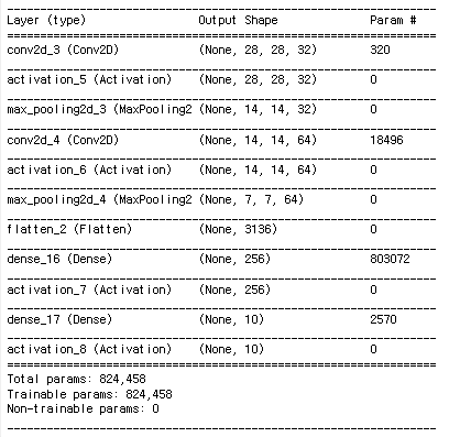
model.summary()
input은 몇개의 영상이 들어갈지 몰라서 none으로 시작, 영상크기, 필터개수 → 파라미터의 개수는 320 (커널크기가 3*3이라서 9개의 가중치를 찾아내야함. 9 + 1(바이어스) , 필터 하나당 10개의 파라미터가 있다. 따라서 320개의 파라미터가 있다.
맥스 풀링 단계로 입력 영상 사이즈만 반으로 줄이는 것으로 14,14,32가된다.
최종 컨벌루션 레이어를 거치면 7*7 64개가 나온다. 1차원으로 Dimension이 나오게 된다.
CNN을 거치면 Dimension커져서 많은 파라미터가 필요해진다.
%%time
hist = model.fit(x_train3, y_train, epochs = 3, batch_size=100)
#batch_size=100은 한번에 전체 영상을 학습하는 것이 아닌 100개씩만 가중치를 업데이트
학습하는 방법은 동일하다.
다양한 층을 거치면서 파라미터를 업데이트 해야하기 때문에 루프를 돌때 시간이 오래걸린다.
이전 방법에 비해 인식률이 높다.
컨볼루션 레이어가 전체 데이터를 잘 분류할 수 있는 특징들을 추출하고 있구나!
plt.plot(hist.history['loss'])
plt.plot(hist.history['accuracy'])
model.evaluate(x_test3, y_test)
일반적으로 2D영상을 인식할 때에는 딥러닝 보단 CNN기반으로 학습시키는 것이 유리하다.
다층 신경망 보다 인식률이 높다.
Deep CNN
model = Sequential()
model.add(Convolution2D(32, (3, 3), padding='same',
input_shape=x_train3.shape[1:]))
model.add(Activation('relu'))
model.add(MaxPooling2D(pool_size=(2, 2)))
model.add(Convolution2D(64, (3, 3), padding='same'))
model.add(Activation('relu'))
model.add(MaxPooling2D(pool_size=(2, 2)))
model.add(Convolution2D(64, (3, 3), padding='same'))
model.add(Activation('relu'))
model.add(MaxPooling2D(pool_size=(2, 2)))
model.add(Convolution2D(64, (3, 3), padding='same'))
model.add(Activation('relu'))
model.add(MaxPooling2D(pool_size=(2, 2)))
model.add(Flatten())
model.add(Dense(128))
model.add(Activation('relu'))
model.add(Dense(10))
model.add(Activation('softmax'))
model.compile(loss='sparse_categorical_crossentropy', optimizer="adam", metrics=['accuracy'])
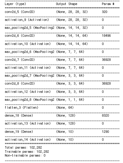
model.summary()
2828 영상이 컨벌루션을 거치면 11로 줄어드게 된다.
필터수가 64개가 되면서 64차원이 된다.
input 영상이 64개밖에 안되기 때문에
첫번째 은닉층을 128로 확장을 해도 충분하다! 따라서 파라미터가 줄일 수 있다.
통상 네트워크를 깊게 설계하면 학습 파라미터의 갯수가 들어가는데
CNN은 맥스 풀링 레이어가 있어 점점 데이터가 줄어든다.
따라서 전체 네트워크의 파라미터 갯수를 줄이는 방법은, 가능한 많은 필터링을 통해 크기를 줄여나가는 것이 좋다.
%%time
hist = model.fit(x_train3, y_train, epochs = 3, batch_size=100)
plt.plot(hist.history['loss'])
plt.plot(hist.history['accuracy'])
model.evaluate(x_test3, y_test)
→ 앞에 CNN 네트워크보다 네트워크 크기가 1/8로 효과적으로 네트워크가 줄었다.
10개의 클래스를 4개의 클래스(상의, 하의, 신발, 가방)로 바꿔서 인식 시키기
a = np.array([1,2,3,3,4,5,6,6])
idx = np.where(a == 2)
#조건에 맞는 인덱스를 찾음
print(idx) #(array([1], dtype=int64),)
print(idx[0]) #[1]
이 방법을 사용할 것
idx = np.where(a > 3) #a>3 인덱스 가져옴
print(idx[0])
#[4 5 6 7]
b = np.zeros(a.shape)
print(b)
b[np.where(a == 3)[0]] = 1   # b[[2,3]] = 1 #a가 3인 부분을 1로 변경
b[np.where(a == 6)[0]] = 2 #a가 6인 부분을 2로 변경
print(b)
b = np.zeros(a.shape)
print(b)
b[np.where(a == 3)[0]] = 1   # b[[2,3]] = 1
b[np.where(a == 6)[0]] = 2
print(b)
y_train_4 = np.zeros(y_train.shape) #y데이터의 크기와 동일한 행렬을 만든다. (모두 0으로)
#상의는 0
y_train_4[  np.where(y_train == 1)[0]] = 1 #하의 경우 레이블 1
y_train_4[  np.where(y_train == 5)[0]] = 2 #5,7,9 신발 레이블 2
y_train_4[  np.where(y_train == 7)[0]] = 2
y_train_4[  np.where(y_train == 9)[0]] = 2
y_train_4[  np.where(y_train == 8)[0]] = 3 #8 가방 레이블  3

y_test_4 = np.zeros(y_test.shape) #테스트 데이터도 마찬가지로 분류
y_test_4[  np.where(y_test == 1)[0]] = 1
y_test_4[  np.where(y_test == 5)[0]] = 2
y_test_4[  np.where(y_test == 7)[0]] = 2
y_test_4[  np.where(y_test == 9)[0]] = 2
y_test_4[  np.where(y_test == 8)[0]] = 3
model = Sequential()

model.add(Convolution2D(32, (3, 3), padding='same',
                 input_shape=x_train3.shape[1:]))
model.add(Activation('relu'))
model.add(MaxPooling2D(pool_size=(2, 2)))

model.add(Convolution2D(64, (3, 3), padding='same'))
model.add(Activation('relu'))
model.add(MaxPooling2D(pool_size=(2, 2)))

model.add(Flatten())
model.add(Dense(256))
model.add(Activation('relu'))

model.add(Dense(4)) #출력층은 4로, 4개의 클래스로 구분하기 때문
model.add(Activation('softmax'))

model.compile(loss='sparse_categorical_crossentropy',
              optimizer="adam",
              metrics=['accuracy'])
%%time
hist = model.fit(x_train3, y_train_4, epochs = 3, batch_size=100)
plt.plot(hist.history['loss'])
plt.plot(hist.history['accuracy'])
model.evaluate(x_test3, y_test_4)
2. ORL Face Recognition, 얼굴 인식 관련 예제 1:00부터 시작
40명에 대한 얼굴인식
orl = fetch_olivetti_faces()
data = orl.data   # 0~1로 정규화 되어 있음.
target = orl.target
print(data.shape)
print(target.shape)
(400, 4096 )
(400, )
데이터의 크기는 400개, 한사람당 10장씩의 데이터로 이뤄져 있다.
d = data[12]
plt.imshow(d.reshape(64,64), cmap='gray')
X_train, X_val, y_train, y_val = train_test_split(data, target, test_size = 0.2)
#80% 학습, 20% 테스트 데이터로 분할
X_train = X_train.reshape(-1, 64, 64, 1) #4차원으로 구성
X_val = X_val.reshape(-1, 64, 64, 1)
input_shape = (64, 64, 1)

model = Sequential()
model.add(Convolution2D(16, kernel_size=(3, 3),
                     activation='relu',input_shape=input_shape))

model.add(MaxPooling2D(pool_size=(2, 2)))

model.add(Convolution2D(32, kernel_size=(3, 3),
                     activation='relu'))
model.add(MaxPooling2D(pool_size=(2, 2)))

model.add(Flatten())
model.add(Dense(512, activation='relu'))    # 512, 1024도 충분
model.add(Dense(40, activation='softmax'))

model.summary()
model.compile(loss='sparse_categorical_crossentropy',        optimizer='adam',     metrics=['accuracy'])
파라미터가 많은 이유 ?
영상의 크기가 크고 (64,64) , 히든 레이어가 512로 파라미터가 크다.
history = model.fit(X_train, y_train , batch_size=20, epochs= 5, verbose=2, validation_data=(X_val, y_val ))
validation_data : 테스트 데이터를 하라는 의미로 20% 테스트 데이터로 validation 하라는 의미
한글인식
r = 0.2
X = np.load('X-h.npy')    # 0 ~ 255, 배경:255,  글자색 0
y = np.load('y-h.npy')

print(X.shape)
print(y.shape)
전체 데이터 샘플 수 는 46060, 영상 이미지의 크기는 32*32 이고 , 3 컬러이미지로 되어있음
plt.imshow( X[33])
X_train, X_val, y_train, y_val = train_test_split(X, y, test_size = r)

print("X_data:", X.shape)
print("y_labels:", y.shape)
print("X_train:", X_train.shape)
print("X_val:", X_val.shape)
print("y_train:", y_train.shape)
print("y_val:", y_val.shape)
학습데이터 : 80%
테스트 테이터 : 20%
X_data: (46060, 32, 32, 3) → 전체 데이터 y_labels: (46060,) X_train: (36848, 32, 32, 3) → 학습 데이터 X_val: (9212, 32, 32, 3) → 테스트 데이터 y_train: (36848,) →각 레이블 y_val: (9212,) →각 레이블
X_train = X_train[:,:,:,0]
X_val = X_val[:,:,:,0]

print(X_train.shape)
3개의 채널 , 컬러는 별로 의미가 없어서 0번째 채널만 사용하겠다
(36848, 32, 32)
plt.imshow(X_train[0], cmap='gray')
그레이로 글자 출력
X_train = X_train.reshape(-1,32,32,1) / 255.0
X_val = X_val.reshape(-1,32,32,1) / 255.0
CNN을 구성하기 위해서 데이터를 4차원으로 reshape, 255로 나눠서 정규화
print("X_data:", X.shape)
print("y_labels:", y.shape)
print("X_train:", X_train.shape)
print("X_val:", X_val.shape)
print("y_train:", y_train.shape)
print("y_val:", y_val.shape)
X_data: (46060, 32, 32, 3) →전체 데이터 y_labels: (46060,) X_train: (36848, 32, 32, 1) → 학습 데이터 X_val: (9212, 32, 32, 1) → 테스트 데이터 y_train: (36848,) →원핫 인코딩 되어 있지 않은 레이블 데이터 y_val: (9212,)
역행렬 기반 학습
X_train2 = X_train.reshape(-1, 32*32) #2차원 -> 1차원
X_val2 = X_val.reshape(-1, 32*32)

y_h = np.eye(980)[y_train] #원핫인코딩, 클래스가 980개

A = np.hstack([ X_train2, np.ones(( X_train2.shape[0]  ,1))  ])
#전체 데이터에서 맨 뒤에 1이 붙은 행렬
print(A.shape)
(36848 , 1025 )
%%time
inv = np.linalg.pinv(A)
W = np.matmul(inv, y_h)
print(W.shape)
(1025 , 980)
1025 는 x번째 클래스를 가장 잘 분류할 수 있는 weight, 클래스 수
A = np.hstack([ X_val2, np.ones(( X_val.shape[0]  ,1))  ])
o = np.matmul(A, W)
print(o.shape) #(9212 , 980 )
p = np.argmax(o, axis=1)
np.mean(p == y_val)
인식이 잘 안됨
이유는 ? 클래스가 많고, 데이터의 분포가 복잡한 비선형 분포를 가지고 있기 때문
CNN 기반 학습
model = Sequential()
model.add(Convolution2D(32, (3, 3), padding='same',
                 input_shape=X_train.shape[1:]))
model.add(Activation('relu'))
model.add(Convolution2D(32, (3, 3)))
model.add(Activation('relu'))
model.add(MaxPooling2D(pool_size=(2, 2)))

model.add(Convolution2D(64, (3, 3), padding='same'))
model.add(Activation('relu'))
model.add(Convolution2D(64, (3, 3)))
model.add(Activation('relu'))
model.add(MaxPooling2D(pool_size=(2, 2)))

model.add(Flatten())
model.add(Dense(512))
model.add(Activation('relu'))
model.add(Dense(980)) #클래스 980
model.add(Activation('softmax'))


model.compile(loss='sparse_categorical_crossentropy', optimizer='RMSProp', metrics=['accuracy'])
%%time
hist = model.fit(X_train, y_train, epochs =10, batch_size=100)
model.evaluate(X_val, y_val)
OpenCV 연동
labels_file = io.open("label.txt", 'r', encoding='utf-8').read().splitlines()
#980개에 대한 레이블 제공

ix,iy = -1,-1
drawing = False
img = np.zeros((256,256), np.uint8) #큰 이미지

def draw(event,x,y,flags,param):
    global ix,iy,drawing, img

    if event == cv2.EVENT_LBUTTONDOWN:
        drawing = True
        ix,iy = x,y

    elif event==cv2.EVENT_MOUSEMOVE:
        if drawing == True:
            cv2.line(img,(ix,iy),(x,y),(255,255,255),15)
            ix = x
            iy = y
    elif event==cv2.EVENT_LBUTTONUP:
        drawing=False


cv2.imshow('image',img)
cv2.setMouseCallback('image',draw)

while(1):
    cv2.imshow('image',img)
    k = cv2.waitKey(1)

    if k == 32 :
        img2 = cv2.resize(img, (32, 32), interpolation = cv2.INTER_LINEAR) #이미지 resize
        plt.imshow(img2, cmap='gray')
        plt.show()

        img2 = 1 - img2.reshape(1,32,32,1) / 255 #배경 글자 색 바꿈 -> predict 시 4차원으로 넣어줌
        id = np.argmax(model.predict(img2))
        print(labels_file[id])
        img = np.zeros((256,256), np.uint8)


    elif k == 27:
        break

cv2.destroyAllWindows()
'Other > Computer vision' 카테고리의 다른 글
| [CV] 객체 검출 Darknet (0) | 2021.12.17 |
|---|---|
| [CV] ImageNet을 이용한 인식 (0) | 2021.12.17 |
| [CV] 사람의 시각을 닮은 신경망 CNN (0) | 2021.12.17 |
| [CV] 전이 학습 (0) | 2021.12.17 |
| [CV] 객체 검출, YOLO (0) | 2021.12.06 |